Methods in Complex Analysis
The Wiener-Hopf Technique
 Wiener and Hopf
An important part of our work in the mathematical study of waves relies heavily on deep results in Complex analysis. In particular, we have a strong expertise in the so-called Wiener-Hopf technique. This technique is very powerful and has been really successful for solving canonical problems exactly for a broad range of applications: acoustics, electromagnetism, elasticity, water-waves, Stokes flows, heat equation, etc. It is traditionally associated to two-dimensional problems and involves functions of one complex variable. Here is a brief historical perspective on the technique.
The essence of the technique consists in using the Fourier transform to pass from a Boundary value problem (PDE + boundary conditions) in the physical space into a functional equation in the complex Fourier space. Such functional equation normally takes the form:
$$\begin{aligned} K(\alpha)\Phi_+(\alpha) = \Phi_-(\alpha) +F(\alpha), \end{aligned}$$ where \(K\) is a known (most often algebraic) function traditionally called the kernel and \(F\) is a known forcing that normally only contains simple poles. The two unknown functions of the problem are \(\Phi_+\) and \(\Phi_-\). It is however normally known that \(\Phi_+\) is analytic in the upper-half \(\alpha\) complex plane, while \(\Phi_-\) is analytic in the lower-half plane.
Often the kernel has a complicated singularity structure, involving branch points, poles, etc. One of the key aspect of the method is to be able to write \(K(\alpha)=K_+(\alpha) K_-(\alpha)\), where \(K_+\) is analytic in the upper half plane and \(K_-\) is analytic in the lower half plane. This is called a factorisation of the kernel. For "simple" diffraction problems involving one infinite scatterers, both the kernel, the unknowns and the forcing are scalar functions. However when multiple scatterers are present, or when scatterers have finite length, the kernel becomes a matrix and the forcing and unknowns are vectors. In this situation, the factorisation (though possible in principle) becomes much more complicated to do in practice and remains an ongoing theoretical challenge.
A few other steps of a similar nature can be done involving the concept of sum-split, and the use of Liouville's theorem. The end result being an exact expression for \(\Phi_+\) and \(\Phi_-\). The physical field can be recovered dierctly via inverse Fourier transform, i.e. a typical complex contour integral. The deformation of contour integration is allowed under certain hypotheses, and chosing the right deformation for optimal evaluation is also of very interesting research topic that we are involved in.
The application of such technique necessitate a very good understanding of functions of one complex variables and their possible singularities, poles, branch points, branch cuts, etc.
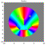
Visualising complex functions is not necessarily straightforward. If one is interested in the location at type of singularities of a function, a simple visualisation tool, called phase portrait can be used.
On such plot, branch cuts are colour discontinuities, and poles and zeroes can also be easily distinguished. Here is an example of such visualisation :)
Here are some of our paper on the topic:
- Nethercote, M.A., Kisil, A.V. and Assier, R.C. (2022)
Diffraction of acoustic waves by a wedge of point scatterers
SIAM journal on Applied Mathematics 82(3), 872-898 - Kisil, A.V., Abrahams, I. D., Mishuris, G. and Rogosin, S.V. (2021)
The Wiener–Hopf technique, its generalizations and applications: constructive and approximate methods
Proc. R. Soc. A 477(2254):20210533, DOI: 10.1098/rspa.2021.0533 - Abrahams, I.D., Huang, X. , Kisil, A.V., Mishuris, G. , Nieves, M. , Rogosin, S. , Spitkovsky, I. (2020)
"Reinvigorating the Wiener-Hopf technique by developing greater insight into the modelling of processes and materials"
National Science Review - Nethercote, M., Assier R.C., Abrahams, I.D. (2020) (open access)
"High-contrast approximation for penetrable wedge diffraction"
IMA J. Appl. Math. 85(3):421-466 (Video) - Nethercote, M., Assier, R.C., Abrahams, I.D. (2020)
"Analytical methods for perfect wedge diffraction: a review"
Wave Motion, 93(102479). - Priddin, M. J. , Kisil, A. V., Ayton, L. J. (2019)
"Applying an iterative method numerically to solve n by n matrix Wiener–Hopf equations with exponential factors"
Phil. Trans. R. Soc. A.37820190241 - Gorbushin, N., Nguyen,V-H., Parnell, W.J. , Assier, R.C. ,Naili, S. (2019)
"Transient thermal boundary value problems in the half-space with mixed convective boundary conditions"
J. Eng. Math. 114 (1): 141-158 - Parnell, W.J., Nguyen, V.-H., Assier, R., Naili, S., Abrahams, I.D. (2016) (open access)
"Transient thermal mixed boundary value problems in the half-space"
SIAM J. Appl. Mathematics 76, 845-866.
Multi-dimensional complex analysis
Generalising the Wiener-Hopf technique to three-dimensional problems would be a tremendous achievement in diffraction theory. However this is far from being straight-forward. One of the reason is that it involves functions that depend on more that one complex variables, such as function on \(\mathbb{C}^2\) or on \(\mathbb{C}^3\) for example, that are 4 and 6 dimensional spaces for example.
In this situation, the singularities of the functions (very important for the WIener-Hopf technique) are not isolated points anymore, but become more complicated geometrical objects. In \(\mathbb{C}^2\) for example, a pole or a branch are objects of real dimension 2.
We are currently doing a lot of work on this topic. In fact a few lectures where given jointly by Raphael Assier and his collaborator Andrey Shanin on this specific topics as part of a Newton Institute programme. These are aimed at applied mathematicians, familiar with one dimensional complex analysis, but keen to know more about the challenges of multi-dimensional complex analysis. Here are the links:
Lecture 1 | Lecture 2| Lecture 3| Lecture 4| Lecture 5
In 2021, Raphael gave another set of three lectures to an AMS even hosted by Harvard University on the topic:
Lecture 1 | Lecture 2 | Lecture 3
Below we present a list of publications on multidimensional complex analysis:
- V.D. Kunz and R.C. Assier (2022)
Diffraction by a right-angled no-contrast penetrable wedge revisited: a double Wiener-Hopf approach
SIAM journal on Applied Mathematics 82(4), 1495-1519 - Assier, R.C. and Shanin, A.V. (2021)
Vertex Green’s functions of a quarter-plane. Links between the functional equation, additive crossing and Lamé functions.
Q.J. Mech. Appl. Math., 74(3):251-295 - Assier, R.C. and Abrahams, I.D. (2021) (open access)
A surprising observation in the quarter-plane diffraction problem
SIAM J. Appl. Math. 81(1), 60-90 - Assier, R.C. and Shanin, A.V. (2021) (open access)
Analytical continuation of two-dimensional wave fields
Proc. Roy. Soc. A, 477:2020081 - Assier R.C., Abrahams, I.D. (2020)
On the asymptotic properties of an interesting diffraction integral
Proc. Roy. Soc. A, 476:20200150 - Assier, R.C., Shanin, A.V. (2019)
"Diffraction by a quarter-plane. Analytical continuation of spectral functions"
Q. Jl. Mech. Appl. Math. 72 (1):51-86 (Video)