PhD student Tom White explains one of the key mathematical tools for understanding complex sound fields.
1. The shape of sound
Sound travels as small vibrations of particles, and can be modelled by a wave of oscillating pressure. A single sound pressure wave is governed by an amplitude and frequency. The amplitude dictates the strength of the pressure wave and the frequency gives the number of full oscillations completed in one second. For a given point in space, the oscillating pressure looks like the following when measured against time:
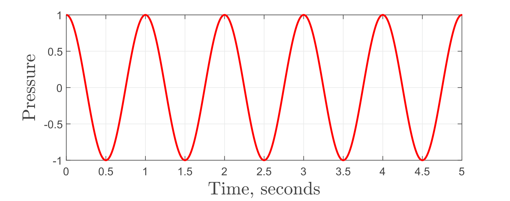
Figure 1. A sound wave with frequency \(f = 1\) and amplitude \(A = 1\).
We can see here that the wave peaks at a pressure of 1, which gives us the amplitude, \(A = 1\), and completes a full oscillation in 1 second meaning the wave has a frequency of \(f = 1\text{Hz}\), and the wave is defined by the cosine function of time, \(t\):
$$ \begin{equation} g(t)=A \cos(2\pi f t) \label{eq:eq1} \end{equation}$$
$$ \begin{equation} g(t)=A \cos(2\pi f t) \label{eq:eq1} \end{equation}$$
A wave of this shape would only produce a simple sound of a single note. In reality the majority of audible sound is the result of many individual waves interacting to create a more complex sound. In Figure 2 we can see how three different sound waves with frequencies \(f = 1, 2\) and \(3 \text{Hz}\) interact to create a sound pressure field.
When the peaks of the waves meet, the pressure field is amplified, and where the the peaks meet the troughs the pressure cancels out. We call this process of overlapping waves to create a non wave-like pressure field superposition. Sound recorded by a microphone is much more likely resemble the pressure field on the right hand side of Figure 2, than the wave in Figure 1. However, for us to look at the complex pressure field it it difficult to identify its component frequencies. In fact, not only can certain sound fields be created by the superposition of waves, but any sound field can be produced by a unique combination of waves.
When the peaks of the waves meet, the pressure field is amplified, and where the the peaks meet the troughs the pressure cancels out. We call this process of overlapping waves to create a non wave-like pressure field superposition. Sound recorded by a microphone is much more likely resemble the pressure field on the right hand side of Figure 2, than the wave in Figure 1. However, for us to look at the complex pressure field it it difficult to identify its component frequencies. In fact, not only can certain sound fields be created by the superposition of waves, but any sound field can be produced by a unique combination of waves.
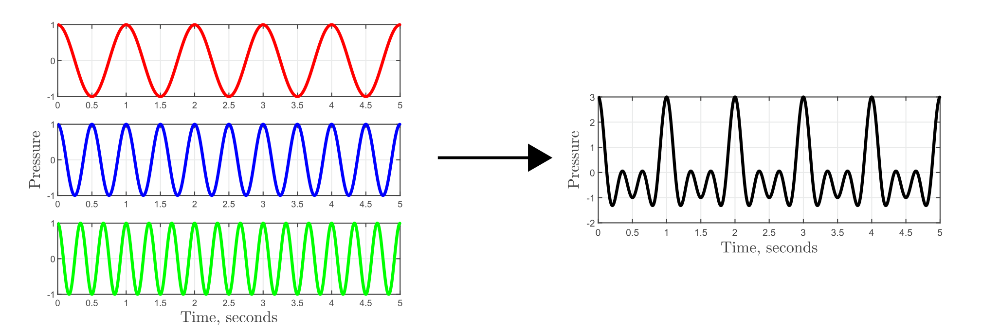
Figure 2. The sum of three waves with frequencies, \(f = 1; 2; 3\text{Hz}\)
2. Fourier Transform
In signal processing and mathematical analysis, it is difficult to analyse a time-pressure field as the individual contributing waves behave independently. For example, different frequencies of sound can be absorbed at different rates by a damping material. Therefore, a tool called the Fourier Transform is used to convert the time-pressure field into a frequency dependent function. The transform was first proposed by a French mathematician, Joseph Fourier, in the 19th century. It converts a time-domain pressure field as discussed above, into a frequency-domain function, which is dependent of the frequency \(f\). The transform is given by the equation
$$\begin{equation} G(f)=\int_\infty^\infty g(t) \exp\{2\pi i f t\}\, dt, \label{eq:eq2}\end{equation}$$
where \(\exp\{-\}\) is the exponential operator, and \( i = \sqrt{-1}\).
$$\begin{equation} G(f)=\int_\infty^\infty g(t) \exp\{2\pi i f t\}\, dt, \label{eq:eq2}\end{equation}$$
where \(\exp\{-\}\) is the exponential operator, and \( i = \sqrt{-1}\).
Initially, the pressure field is given as a time-domain function, where the pressure changes over time. However, after the Fourier transform is applied, this dependence on time is removed, and the solution becomes a function of frequency, peaking where there are contributing frequencies. An important property of the Fourier transformed function is that the sum of two Fourier transforms is equal the Fourier transform of the sum of two waves. Therefore, we can analyse the behaviour of our Fourier transformed function as sound behaves differently at each frequency, and then transform the final product back into the time domain to get the resulting sound field.
In Figure 3 the first graph shows the resulting field of three waves in superposition, with frequencies \(f = 1/2\pi\), \(f = 1\) and \(f = 2\), given by
$$\begin{equation} g(t)=2\cos(t)+\cos(2\pi t)+\cos(4 \pi t). \label{eq:eq3}\end{equation}$$
In Figure 3 the first graph shows the resulting field of three waves in superposition, with frequencies \(f = 1/2\pi\), \(f = 1\) and \(f = 2\), given by
$$\begin{equation} g(t)=2\cos(t)+\cos(2\pi t)+\cos(4 \pi t). \label{eq:eq3}\end{equation}$$
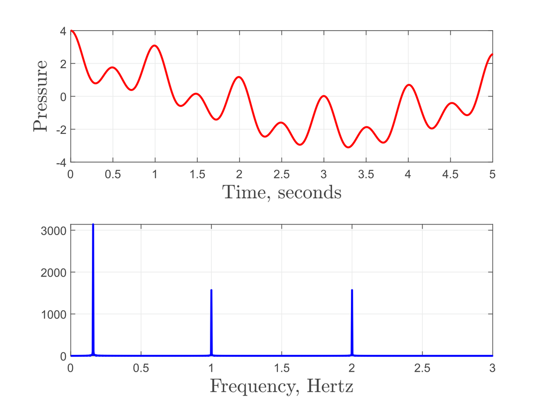
Figure 3. Fourier Transform of \(f = \cos(2\pi t) + \cos(4\pi t) + 2 \cos(t)\).
The second graph in Figure 3 shows the Fourier transform of \((\ref{eq:eq3})\). The Fourier transform clearly has spikes at the three contributing frequencies in f, and the relative height of the spikes tells us about the relative strength of each wave to each other. In the initial function \((\ref{eq:eq3})\) we see that the \(f=1/2\pi\) wave has twice the amplitude in as the other two contributing waves, which is reflected in the Fourier transform, with the spike at this frequency being twice as large. The inverse Fourier transform can also be performed, to create a sound profile from a given frequency domain function.
3. Applications of the Fourier transform
In sound analysis the Fourier transform is very useful in helping us understand the composition of sound and how it changes as it passes through certain materials. This is because each sound frequency behaves differently in different materials, so to understand how a given sound changes we must first know which frequencies are contributing to the sound profile. The transform is also very useful in sound editing. If, for example you wanted to remove a high pitched noise from a recording, by taking the Fourier transform the high pitched frequency can be identified. Then by 'squashing' the peak at this high frequency and performing the inverse Fourier transform to return to a time-domain signal, the high pitched note will have been removed.
The Fourier transform is not limited to use in sound processing and analysis: it can be applied to any system where there is known to be an oscillating energy source which can operate at a continuous spectrum of frequencies. For example, the Fourier transform is used in a wide range of spectroscopy techniques such as Nuclear Magnetic Resonance (NMR) spectroscopy which uses the Fourier transform to analyse the magnetic fields of atomic nuclei.
The Fourier transform is not limited to use in sound processing and analysis: it can be applied to any system where there is known to be an oscillating energy source which can operate at a continuous spectrum of frequencies. For example, the Fourier transform is used in a wide range of spectroscopy techniques such as Nuclear Magnetic Resonance (NMR) spectroscopy which uses the Fourier transform to analyse the magnetic fields of atomic nuclei.
 RSS Feed