PhD student Eleanor Russell discusses an important concept in the development of robust advanced materials
1 Inclusions: The good, the bad and the ugly
In material science, we refer to a material domain as a matrix and an inclusion as an object inside the matrix with different material properties.
| Inclusions of all different shapes and sizes can be used to intentionally alter the effective properties of a composite material. For example, reinforcing brittle concrete with steel rods to increase its strength or, on a smaller scale, embedding highly conductive fibres throughout a less conductive matrix to improve heat dissipation. In both cases, the material properties of the matrix and inclusions complement each other and result in a more practical composite material. On the other hand, sometimes engineers are forced to incorporate inclusions into their designs; adding windows along the side of commercial aircraft for instance. In this case, the material properties can be affected in undesirable (and occasionally catastrophic) ways. | 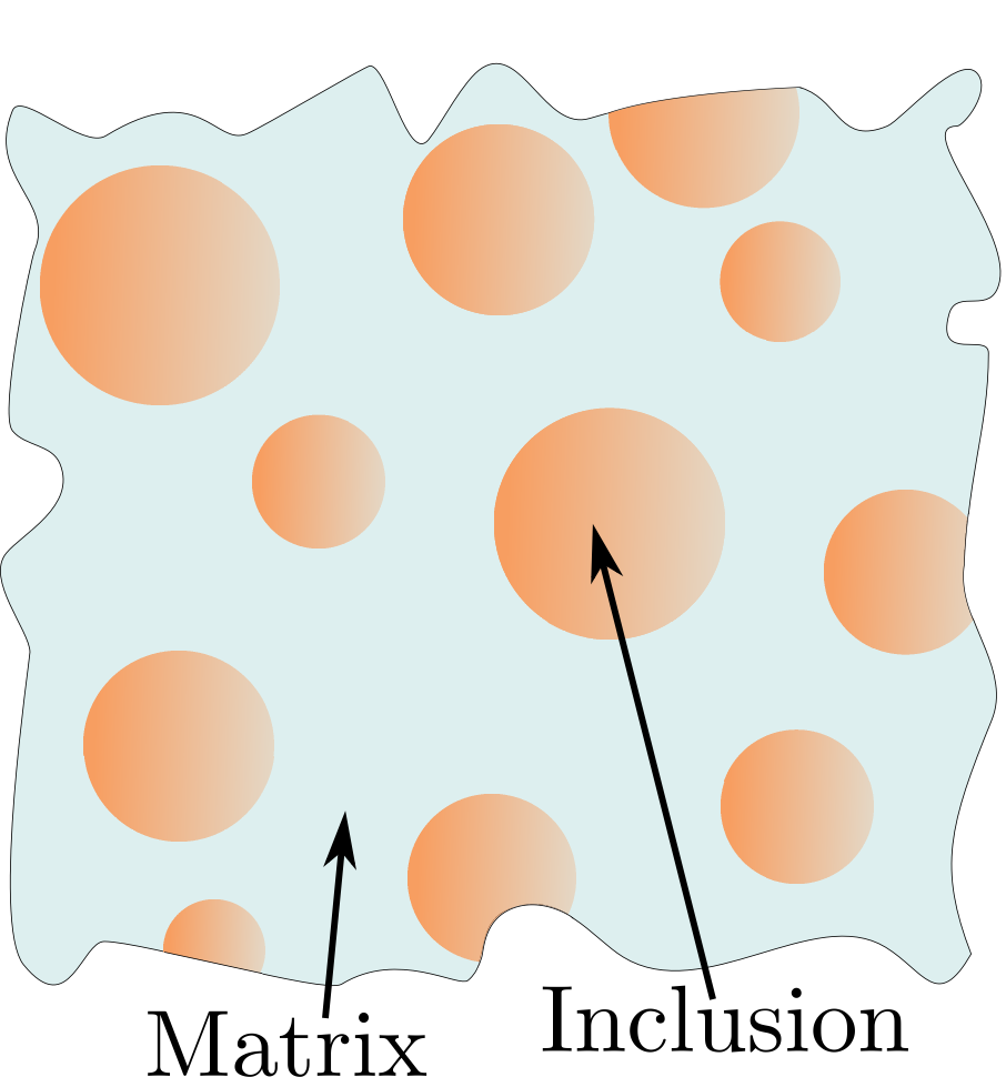 |
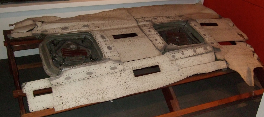 Fragment of the first production Comet at the Science Museum in London. Image credit: Krelnik, CC BY-SA 3.0 | A famous example is the world's first jetliner, the Comet, in 1952. The pressurised cabins were designed with large, squared-off windows causing pressure to repeatedly build-up at the corners. At high altitudes the corners of a window could be subjected to pressure up to three times higher than the rest of the cabin. Unfortunately, in several cases, this resulted in fatal structural damage. To avoid this problem, aircraft are now designed with the rounded, porthole-style windows we see today, however, neutral inclusions could offer an alternative approach. |
2 Neutral Inclusions
Neutral inclusions were first introduced by Mansfield in 1953 for holes in plates [1]. The idea is to provide inclusions with an additional coating to remove any undesired perturbations from the physical fields in the matrix. A perturbation is any deviation of a field from its state when the inclusion is not present.
| For example, we could surround the squared-off windows of the Comet with an additional coating to relieve the pressure from its corners. The required properties of the coating will depend on both the matrix (the cabin wall) and the inclusion (the window). If the necessary properties are satisfied the combination of the inclusion and its coating is referred to as a neutral inclusion and the fields in the matrix become unperturbed. All we need now is to determine the required properties within the coating. To show how we approach this problem we consider perturbations within the temperature field of a matrix. | 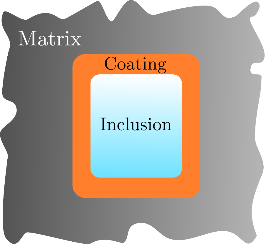 |
2.1 Neutral Inclusions: thermal conductivity example
In the following example we consider a steady-state, two-dimensional problem. The steady-state assumption removes any time-dependence from the solution. As a result, the only material property we need to consider is the thermal conductivity, denoted \(k\). The thermal conductivity of a material measures its ability to conduct heat through diffusion.
We are interested in the temperature field, \(T(\mathbf{x})\), which must satisfy the heat equation. For this example, we assume the thermal conductivity is isotropic (independent of direction) and homogeneous (independent of position) and is therefore a scalar. As a result, together with the steady-state assumption, the heat equation reduces to Laplace's equation, given by:
$$\begin{equation}
\nabla ^2 T(\mathbf{x}) = 0,
\label{laplace}
\end{equation}$$
where \(\nabla ^2\) is the Laplace operator.
Consider the linear temperature field in Figure 1, where the black lines represent lines of constant temperature called isotherms. This temperature field is linear with respect to \(x\) and therefore has the form \(T(x)=\alpha x+\beta\) for some constants \(\alpha\) and \(\beta\).
Let the matrix in Figure 1 have conductivity \(k_m\). Notice in Figure 2 that when a circular inclusion with conductivity \(k_i\), where \(k_i \neq k_m\), is embedded in the matrix, the field becomes perturbed and is no longer linear.
Let the matrix in Figure 1 have conductivity \(k_m\). Notice in Figure 2 that when a circular inclusion with conductivity \(k_i\), where \(k_i \neq k_m\), is embedded in the matrix, the field becomes perturbed and is no longer linear.
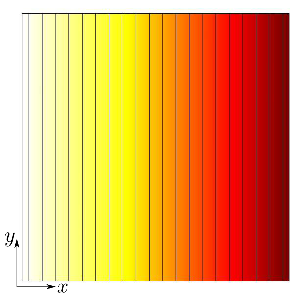 Figure 1: Linear temperature field with respect to x-coordinate | 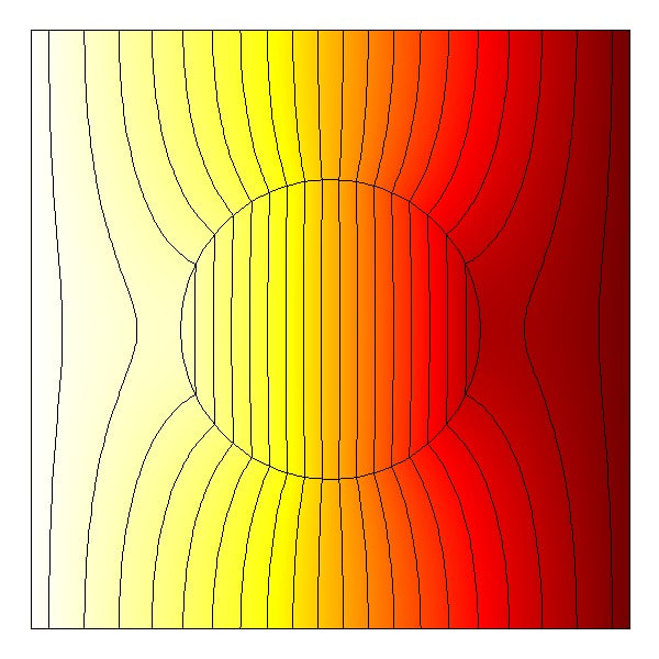 Figure 2: Inclusion leading to perturbations |
By adding a coating with conductivity \(k_c\), as illustrated in Figure 3, we can remove the perturbations from the matrix and recover the linear temperature field
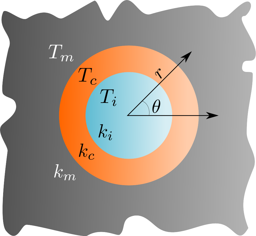 Figure 3: Configuration for neutral inclusion in polar coordinates, x = [r,θ]. | The temperature fields in the matrix, coating and inclusion are denoted by \(T_m(\mathbf{x}),\ T_c(\mathbf{x})\) and \(T_i(\mathbf{x})\) respectively and must all satisfy Laplace's equation. We solve (1) for all temperature fields to find: $$ \begin{equation} \begin{split} &T_m(r,\theta) = \left(\alpha r + \dfrac{B_m}{r}\right) \sin \theta, \\ &T_c(r,\theta) = \left(A_c r + \dfrac{B_c}{r}\right) \sin \theta, \\ &T_i(r,\theta) = A_i r \sin \theta, \label{temp fields} \end{split} \end{equation} $$ where \(B_m,\ A_c,\ B_c\) and \(A_i\) are constants. |
We wish to find a solution where \(B_m=0\) as this leads to a linear temperature field throughout the matrix given by \(T_m(r,\theta)=\alpha r \sin \theta = \alpha x\) (since \(x=r \sin \theta\)).
Let the radius of the inclusion and coating be given by \(r_i\) and \(r_c\) respectively. Solving the temperature fields in (2) with perfect contact conditions across each interface (continuity of heat flux and temperature) we find that \(B_m=0\) is satisfied when
\begin{equation}
D^2 = \dfrac{(k_m-k_c)(k_i+k_c)}{(k_i-k_c)(k_m+k_c)} \qquad \text{where} \qquad D= \dfrac{r_i}{r_c}
\label{k cond}
\end{equation}
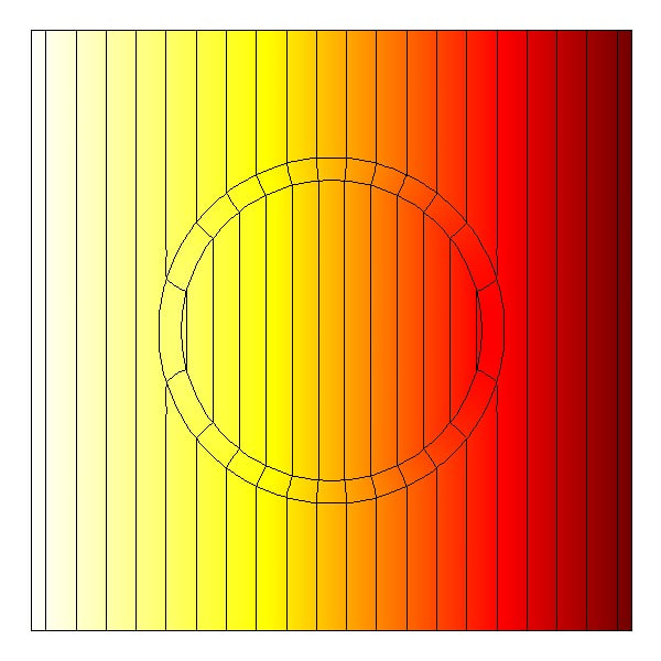 Figure 4: Neutral Inclusion leading to unperturbed field in the matrix
 Therefore, the two radii and the conductivities of all three components are dependent on each other. Figure 4 shows the resulting temperature fields when the condition in (3) is satisfied. We see that the temperature field in the matrix is unperturbed and once again linear with respect to \(x\) as required.
2.2 Neutral inclusions: extensions and limitations
As we are not restricted to a single coating, we can extend the work in the previous section with as many additional coatings as we wish. For example, a bi-layer neutral inclusion where an inner coating insulates its core region, protecting the inclusion from external forces, and an outer coating counteracts any perturbations caused by the insulator. Since the inclusion may have any material properties, the bi-layer neutral inclusion acts as a cloak for the specific problem it is designed for.
In terms of limitations, firstly, an isotropic solution may not exist for a given field. For example, to find a neutral inclusion for a pressure field we must relax the isotropic assumption. Secondly, a neutral inclusion is not a perfect cloak as it is tailored for a specific configuration with fixed external forces. Therefore, if we change the nature of the external forces, the properties within each coating will no longer achieve the desired effects.
A perfect cloak is one which, regardless of the external forces, leads to unperturbed fields in the matrix. Transformation theory is used to design perfect cloaks and other interesting concepts. We will discuss these in a future blog post.
A perfect cloak is one which, regardless of the external forces, leads to unperturbed fields in the matrix. Transformation theory is used to design perfect cloaks and other interesting concepts. We will discuss these in a future blog post.
[1] E. H. Mansfield, Neutral holes in plane sheet - reinforced holes which are elastically equivalent to the uncut sheet, The Quarterly Journal of Mechanics and Applied Mathematics, 1953, 6(3), 370–378
 RSS Feed